On Different Perspectives of Measuring Data Utility
July 31, 2023
Overview
Modern Deep Neural Networks are trained on a massive amount of data. Numerous works have proposed methods to estimate the contribution of each single datapoint. There are various ways to do this: to begin with, we can use hardcoded heuristics. For example, using sentence length and word frequency to determine whether a particular sentence is hard for a language model to learn. This method might seem hacky, but even the latest research on machine translation/language generation designs hardcoded heuristics based on the relative position of the token [Liang et al., 2021, Jia et al., 2023]. These methods usually induce numerous extra hyper-parameters and thus require careful tuning for performance. More importantly, relying on a task-specific heuristic does not generalize well to new tasks without domain-specific knowledge. I will not review the details of these methods in the blog post and instead focus on ways that show promises of generalization beyond the tasks the authors experimented on.
There are also lines of work that are more theoretically grounded by approximating the influence on training and validation loss of each datapoint. These lines differ in their way of doing this approximation. In this blog post, I will go over each of these methods and discuss each method’s strengths and limitations. This blog post also covers my thoughts on connecting data utility evaluation with curriculum learning and studies on the loss landscape.
At last, I will cover some of my latest thoughts for future directions. Research on data quality estimation traces back to the mid-90s but is still rapidly evolving. It would be crucial to design more efficient methods when the model and data sizes are scaling up exponentially.
Dataset Pruning:
A canonical way of estimating the contribution of individual parameters is by how much the training loss is affected when the parameter is removed. Similarly, we can also measure how the change of the loss is affected when a single datapoint is removed in a single batch.
Paul et al., 2021 approaches this problem by analyzing the change in loss when the update steps are continuous: The time derivative of the loss for a given training example is given by:
Where $S$ is the mini-batch in SGD or the entire training set in GD.
Intuitively, the metric $\Delta_t ((x, y), S)$ measures the change in training loss when using an infinitesimal learning rate - the gradient flow. Now we bound the difference in loss of any example with an infinitesimal learning rate.
Theorem: Up to a constant $c$, the change in loss for another example in the same batch under an infinitesimal learning rate setting when a specific datapoint in that batch is pruned is bounded by the gradient norm of that pruned example:
$\|\Delta_t((x,y),S) - \Delta_t((x, y), S_{\neg j})\| \leq c\|g_t(x_j, y_j)\|$
Please refer to the paper for detailed proof.
However, it is hard to calculate the gradient for a single example at training iteration $t$: $g_t(x_j, y_j)$ since we batch multiple training examples together and aggregate the gradients. If we assume that the gradients of each logit $\nabla w_t f_t^{(k)}(x)$ are orthogonal and have similar sizes, we can approximate the per example gradients as:
The R.H.S is the $\ell_2$ norm of the error vector. The paper calibrates the error l2 norm (EL2N) with multiple training runs at a specific training iteration. The author finds out that the model can identify hard training examples/noise in data with a very high EL2N score, and pruning 40% to 50% percent of data in CIFAR10 and 20% to 30% of data in CIFAR100 matches the performance of full training.
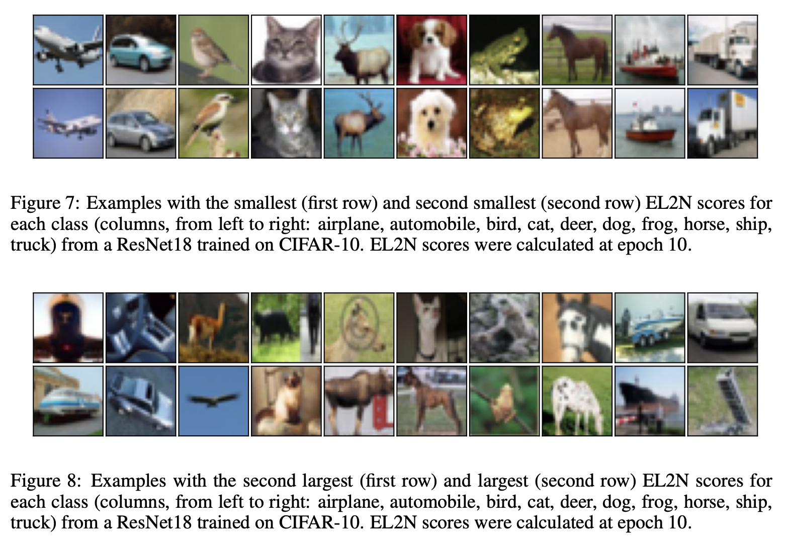
EL2N scores (l2 norm of prediction vector - groundtruth one-hot vector) are highly effective in identifying data that are either too hard or contain noise (see the following picture from the paper for easy and hard examples in image classification).
However, one intriguing question is how we can know that the high error norm for a datapoint correctly identifies a certain datapoint as noise instead of the model being incompetent. Choosing the EL2N score of arbitrary checkpoints and testing out performance does not scale well to large datasets. Another question I had was how this method generalizes to tasks other than image classification. I tested out this dataset pruning method on a multilingual machine translation task by selecting four language pairs (en-{de, es, fr, it}) from the opus-100 dataset:
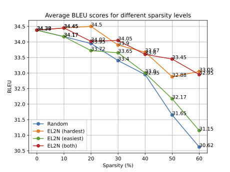
Although I only did one training run for each pruned sparsity, the difference between pruning high EL2N and random pruning is high, especially when more data is pruned, showcasing that this method generalizes well under a machine translation setup. But what is more interesting is that for machine translation, the maximal percentage of data you can prune without harming the performance is around 20% as opposed to the 30%-40% redundancy in image classification - which is counterintuitive because machine translation data, from my perspective, should be noisier than image classification data and thus a higher percentage of data can be pruned.
I want to wrap this section of this paper up by re-iterating the limitation of this method: calibration of the EL2N score requires several training runs. For classification tasks with only a few labels, this is not a problem as a single or a few runs might give you a reasonable estimate. However, in language modeling, where the label size is your dictionary’s size, the variance of EL2N is high. It thus requires trying out different iterations and multiple training runs for a more accurate estimate.
Sorscher et al., 2022 presents a follow-up work by proposing to cluster the data using their representations in a pre-trained model (in the paper, they used the SWaV model on ImageNet) and find examples that are super far away from the clusters to detect data to prune. Directly applying this to language modeling or machine translation raises the problem of having a large number of clusters. In ImageNet, there is only 1000 classes resulting in 1000 cluster centers, whereas in language modeling, the vocabulary size is at least $20 \times$ large.
However, suppose dataset pruning can beat scaling laws: we can train much better LMs without exponentially increasing the amount of data by applying unsupervised clustering methods on text. In that case, this research direction should be promising. The question remains how can we automatically filter high-quality data from the enormous amount of data we have and validate that the data we have is high quality without full training runs of large language models - is training a tiny LM on high-quality data sufficient for validating the quality of data?
Influence Functions
Another line of work [Koh and Liang, 2017, Pruthi et al., 2020, Yang et al., 2023] also estimates data utility by how much of a difference it makes when that specific datapoint is removed. However, instead of measuring the difference in loss as in the aforementioned works, they measure the difference in the parameters. Formally, if $\hat{\theta}$ and $\hat{\theta}_{\neg z}$ are the empirical risk minimizers of the training set with and without a certain datapoint $z$, respectively, we measure the difference to represent the utility of the datapoint $z$:
Statistical theory [Cook and Weisberg, 1982] gives us an approximation of change in parameters if a certain example is upweighted by a factor of $\epsilon$ . This is equivalent to training on this augmented loss: $\frac{1}{n} \sum_{i=1}^n \mathcal{L}(z_i, \theta) + \epsilon \mathcal{L}(z, \theta)$.
Setting the upweighting factor to $\epsilon = -\frac{1}{n}$ is the same as removing the datapoint, therefore we approximate the utility of the datapoint by
Ultimately we care about the test performance. Applying the chain rule, we can also approximate the change of the test loss when a particular training example $z$ is removed:
Here we are able to see that the difference in test loss is also upper bounded by the norm of the gradient on that particular training example scaled by constant factors. Moreover, it also shows whether pruning a particular example would improve or degrade test performance depends on the dot product between the training and test gradients - this is intuitive. Still, in practice, we cannot access the test set. Numerous works have used the dot product between the training gradient and development gradient as a proxy for data utility [Wang et al., 2020a, Wang et al., 2020b, Yang et al., 2021]. Therefore, the influence function here takes three things into account for estimating data utility:
- The similarity between training and test gradients $\nabla_\theta\ell(z_\textrm{test}, \theta)^\top \nabla_\theta\ell(z, \hat{\theta})$;
- The local curvature of the loss function at the current training step $\mathcal{H}^{-1}_{\hat{\theta}}$;
- The magnitude of training gradient: $\|\nabla_\theta\ell(z, \hat{\theta})\|$.
In theory, this should be a more accurate estimate, but this method is impractical as it requires us to compute the per-sample gradients, which is already expensive. Not to mention calculating the dot product and the Hessian during every training iteration.
Recent work reframes data selection as two discrete optimization problems [Yang et al., 2023]:
- Given a constraint on the change in the norm of parameters, find the largest subset of data that satisfies this constraint.
- Given the budget on the fraction of data to prune, find the subset of data that results in the minimal change in parameters.
The essence of this method is that they consider the “group effect” when pruning data. One datapoint might have large gradient norms that seem unprunable, but when combined with another datapoint, they have a small gradient norm and can be pruned together. In the paper, the author solves the optimization problem with simulated annealing [Van Laarhoven and Arts, 1987]. A critical engineering trick to speed up estimation is only computing the influence on the last linear layer.
Connections with Curriculum Learning
So far, we have assumed that the utility of a single datapoint is static and model agnostic. These methods pre-compute the utility of data, filter out the noisy ones, and launch another training run on the pruned dataset. But in fact, the estimations (EL2N or Influence Functions) take the models’ current states into account so they should be dynamic. A naive connection would apply this to curriculum learning, where each datapoint is assigned a score and presented to the model adhering to a given schedule.
The motivation is that humans learn knowledge at different paces and models as well [Wu et al., 2021], so we should present the easier data first, then more complex data, or general domain data first, then in-domain data. Existing research of curriculum learning for machine translation/language modeling ranks the training data with pre-defined heuristics. e.g., the perplexity of the text when evaluated by a trained language model [Moore and Lewis, 2010], sentence length and averaged word frequency [Platanios et al., 2019], similarity to the in-domain data [Zhang et al., 2019]. On a token level, this can be the position of the token [Liang et al., 2022, Jia et al., 2023].
However, the schedule of how we should present the data stream with different scores is not well studied. The above work usually handcrafts several schedules and tests them out empirically, inducing many additional hyper-parameters to test out. Suppose we apply the pruning metrics which considers the model’s current state, we can design automated curriculums without pre-defined metrics or requiring a handcrafted schedule.
Future Directions
Moving forward, I think there are some promising research directions that are worth exploring:
- Dataset Pruning on large scale text corpora: So far, all of these dataset pruning papers experiment on the task of image classification data, but does the findings still hold when evaluated on datasets that are magnitudes larger? How can we adapt these methods to language modeling/machine translation if not?
- The theory behind curriculum learning: Why does presenting the data in a given order speeds up training or have better generalizability? Does it guide the model to a smoother area in the loss landscape?
- Evaluating models beyond test loss: Does the distribution of data quality estimated by the model also give an estimate of the model itself?